Statistics as a Language
STAT 240 - Fall 2025
Statistics as a Science
The Scientific Method
- Where does statistics come into the picture?
\[ \begin{array}{|c|} \hline \text{Observe}\\ \hline \text{Question}\\ \hline \text{Hypothesize}\\ \hline \text{Experiment}\\ \hline \text{Analyze}\\ \hline \text{Conclude}\\ \hline \end{array} \]
Observe and Question
Tsunamis can occur after earthquakes
They tend to happen after high magnitude earthquakes
How high magnitude does an earthquake have to be to cause a tsunami?
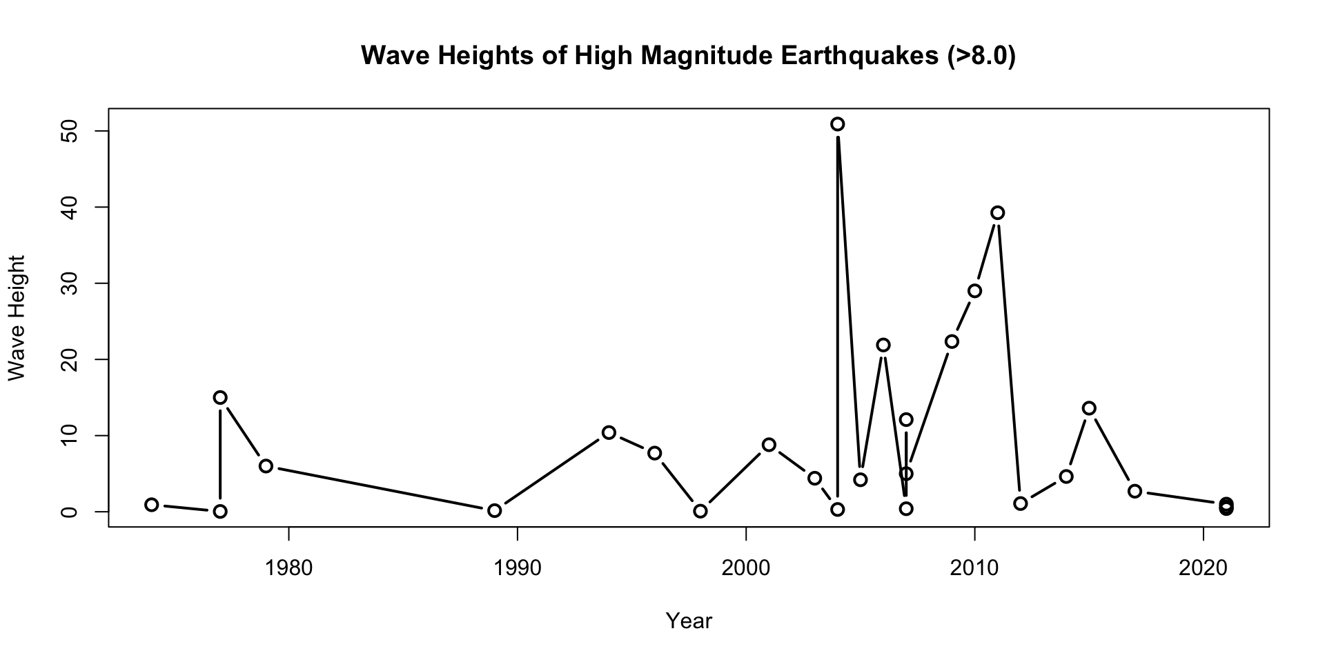
How high are the tsunami waves from high magnitude earthquakes?
Hypothesize
“On 30 July 2025, at 11:24:52 PETT (23:24:52 UTC, 29 July), a \(M_w\) 8.8 megathrust earthquake struck off the eastern coast of the Kamchatka Peninsula in the Russian Far East, 119 km (74 mi) east-southeast of the coastal city of Petropavlovsk-Kamchatsky.” – Wikipedia
This earthquake was well above the severity to cause a tsunami
Higher magnitude earthquakes result in tsunamis with high waves
Experiment
We can’t experiment well with this kind of science
But we can run a sort of “psuedo”-experiment
We select \(100\) tsunamis at random and see if they were the product of an earthquake
We find out that \(68\) of them had some connection to a earthquake
Vocabulary (Get used to it)
Population: the entire collection of individuals about which information is sought.
Sample: a subset of population, containing the individuals that are actually observed.
Statistics: is the study of procedures for collecting, describing, and drawing conclusions from information.
- the science of describing or making inferences about a population, from a sample.
Analyze
Of the 748 tsunamis that have occurred since 1970, 464 of them can be directly associated with an earthquake.
From this data we can say two things
\(62\%\) of tsunamis are caused by earthquakes
\(68\%\) of the tsunamis in our sample were caused by earthquakes
Parameter: a value that describes an entire population.
Statistic: a value that describes a sample.
Sampling Techniques
I hope you’re hungry
Simple Random Sampling
How clean are the campus dining halls? Let’s find out!
We decide to line up all of the dining hall workers at Kramer
Everyone is assigned a number, \(1\) to \(50\)
We randomly select \(10\) numbers
Then swab the hands of every person who’s number came up
Simple Random Sampling
Simple Random Sample (SRS): a sample chosen by a method in which collection of n population items is equally likely to make up the sample.
Every worker had the same chance of being selected
\(1/50\)
Note: this only works if we select all \(10\) numbers simultaneously
We’ll play with that concept more later on
Stratified Sampling
Maybe the \(10\) workers we selected all work the same station together. How can we make sure we get a sample from every station?
Divide up workers by station, \(5\) in total
Assign each group of workers numbers \(1\) through \(10\)
Randomly select \(2\) numbers
Swab the hands of each of those numbers from each group
Statified Sampling
Stratified Sample: The population is divided into groups, called strata, where the members of each stratum are similar in some way. Then a SRS is drawn from each stratum.
We stratified by station
We defined a SRS for the strata
We sampled from the strata based off of that SRS
Cluster Sampling
Foodborne outbreaks can also happen as a result of contaminated regions, not just bad worker hygeine.
We split the dining center up into a grid of 5 ft by 5 ft squares
We select \(10\) squares at random and swab the entire square
Each of these squares are called clusters
Cluster Sampling: Items are drawn from the population in groups, or clusters.
Systematic Sampling
At the end of the day, the delivery mechanism of foodborne illness is the food itself.
We decide to sample the food coming off the line directly
It’d be a massive interruption of service to sample every food item coming out
- Plus, we can’t serve food once we’ve sampled it
So we decide to sample every \(10^{th}\) item that comes from any station for possible contaminants
Systematic Sampling
Define a number, denoted \(k\)
Sample the \(k^{th}\) item that’s observed
Repeat the sampling process every \(k\) items that are observed
Voluntary Response
We design a simple survey that asks the students:
On a scale of 1 to 10 how clean does Kramer dining center appear?
Have you ever felt sick after eating at the dining center?
Do you think the dining center prioritizes food safety adequately?
We send the survey to every student that’s eaten at Kramer in the past year
Samples of Convenience
How does the class feel about Kramer on a scale of 1 to 10?
It an easy sample to acquire, we just used who we had
It’s a terrible sampling technique in general
Why?
Data Types
Data
What is data?
Data: Information that has been collected
Individual: Something the information has been collected on (People/Places/Things/etc.)
Variables: Characteristics about the individuals we collected information (data) from
Variables
\[ \scriptsize \begin{array}{|c|c|c|c|c|c|} \hline \textbf{Location of harvest} & \textbf{Date of harvest} & \textbf{Sex} & \textbf{Age class} & \textbf{Body mass in kg} \\ \hline \text{Boyer} & 2005\text{-}10\text{-}15 & \text{Female} & 3.5 & 34.0 \\ \text{Desoto} & 2004\text{-}12\text{-}12 & \text{Male} & 3.5 & 71.2 \\ \text{Desoto} & 2009\text{-}10\text{-}17 & \text{Male} & 0.5 & 21.8 \\ \text{Desoto} & 2010\text{-}01\text{-}02 & \text{Male} & 0.5 & 19.5 \\ \text{Desoto} & 2005\text{-}12\text{-}11 & \text{Female} & 3.5 & 45.4 \\ \hline \end{array} \]
Not all variables are held equal
What’s the difference between column 1 and column 2?
- What about 3 and 4?
Categorical Variables
Qualitative (Categorical) variable: The value of the variable represents a descriptive categories
Identifying labels or names
We can’t really do math with a label or name
“Male” \(= 0\), “Female” \(= 1\)
Categorical Variables
Ordinal variables: Categories/values of the variable have a natural ordering
Letter grade: A, B, C, D, F
Age classifications: Young, Middle-aged, Old
Nominal variable: Categories/values of the variable cannot be ordered naturally
Degree program
Sex: Male / Female
Numeric Variables
Quantitative variable: The value of the variable represents a meaningful number
Body mass, age, height, time
We can inherently do math with these
Can still be problematic due to units
Numeric Variables
Discrete variable: A countable number of values (0, 1, 2, 3, 4, …)
Population size of fish in a pond
How many times a coin flip was successfully called
Continuous variable: A continuous range of numbers (0, 0.1, 0.11, 0.111, …)
Temperature
Volume of liquid in a glass
Body Mass
Numeric Variables
Interval level
Differences between values make sense
Ratios don’t make sense because zero has no meaning
Ratio level
Differences between values make sense
Ratios also make sense
Zero has meaning, it represents absence of the quantity
Summarizing Data
Frequency Distribution
Statistics is really good at summarizing grotesque amounts of information
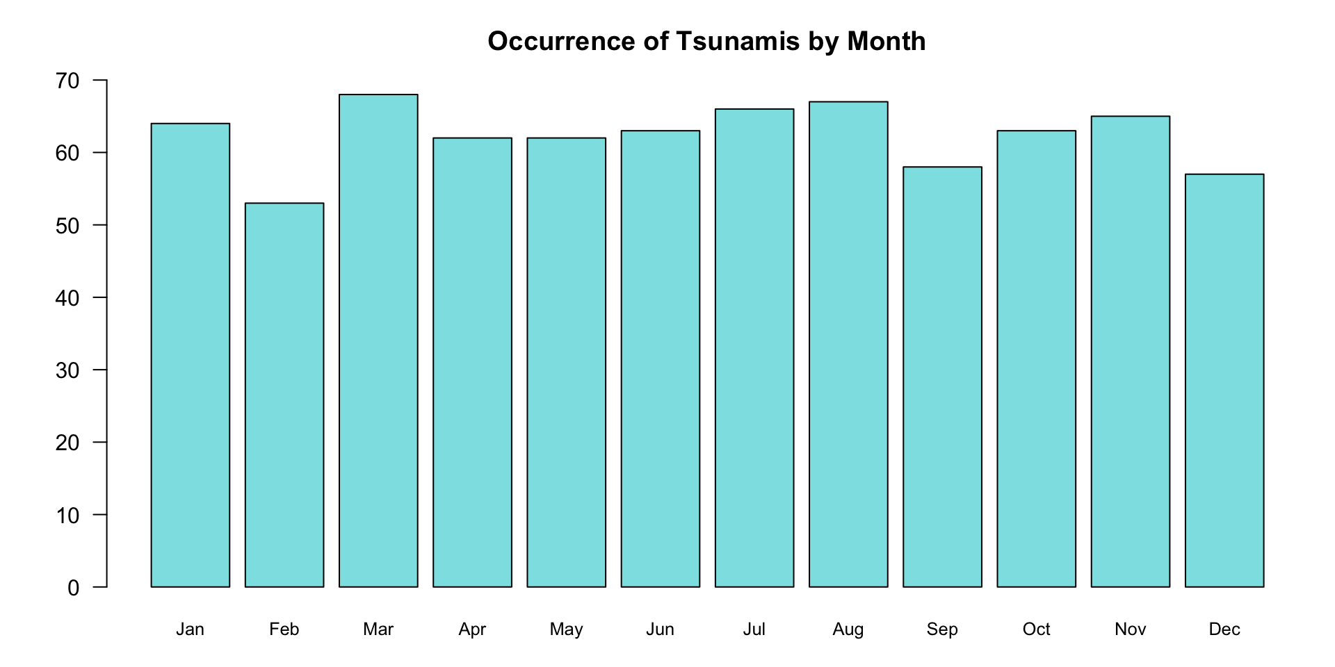
Of the \(748\) tsunamis that have occurred since 1970, when do they usually occur?
We can look at the months, since exact date is a little impractical
Instead of a table of raw data, we can just record each time a specific month appears
Frequency Distribution
Frequency distribution:
Groups data into categories
Records the number of observations that fall into each category
“How frequently do these variables occur in my sample?”
\[ \begin{array}{|c|c|c|c|c|c|c|} \hline \text{Month} & \text{Jan} & \text{Feb} & \text{Mar} & \text{Apr} & \text{May} & \text{Jun} \\ \hline \text{Frequency} & 64 & 53 & 68 & 62 & 62 & 63\\ \hline \text{Month} & \text{Jul} & \text{Aug} & \text{Sep} & \text{Oct} & \text{Nov} & \text{Dec}\\ \hline \text{Frequency} & 66 & 67 & 58 & 63 & 65 & 57 \\ \hline \end{array} \]
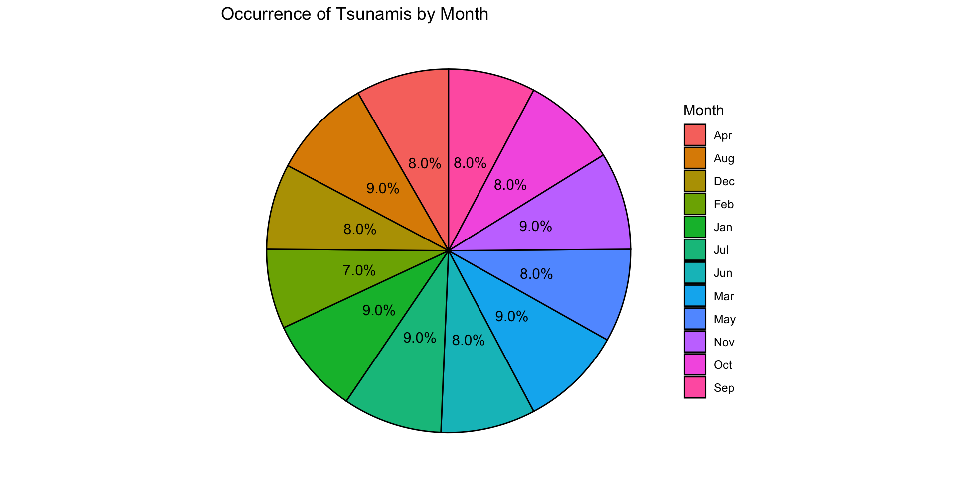
Relative Frequency
Relative frequency distribution
Divide the frequency by the total observations
This gives us the proportion of units in each category
“What percentage of my sample is this category?”
\[ \begin{array}{|c|c|c|c|c|c|c|} \hline \text{Month} & \text{Jan} & \text{Feb} & \text{Mar} & \text{Apr} & \text{May} & \text{Jun} \\ \hline \text{Frequency} & 64 & 53 & 68 & 62 & 62 & 63\\ \hline \text{Relative Frequency} & 0.09 & 0.07 & 0.09 & 0.08 & 0.08 & 0.08\\ \hline \text{Month} & \text{Jul} & \text{Aug} & \text{Sep} & \text{Oct} & \text{Nov} & \text{Dec}\\ \hline \text{Frequency} & 66 & 67 & 58 & 63 & 65 & 57 \\ \hline \text{Relative Frequency} & 0.09 & 0.09 & 0.08 & 0.08 & 0.09 & 0.08 \\ \hline \end{array} \]
Numeric Frequency
We can do the same thing with numeric values
If we wanted to group the tsunamis caused by earthquakes by magnitude of earthquake
We’d need to define some kind of classification for earthquake magnitude
Then we could sort them by that
Let’s say: \(0.0-0.9\), \(1.0-1.9\), …
Numeric Frequency
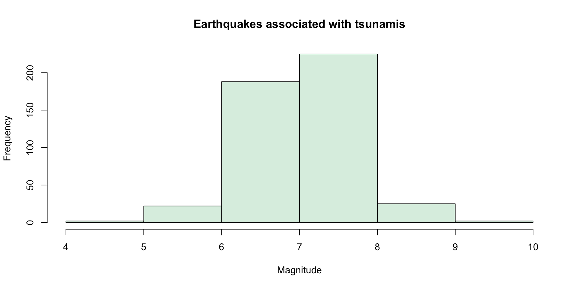
There were no tsunamis caused by earthquakes less than a magnitude of 4, so we can remove those classes
\[ \begin{array}{|c|c|c|c|c|c|c|} \hline \text{Class} & 4.0-4.9 & 5.0-5.9 & 6.0-6.9 & 7.0-7.9 & 8.0-8.9 & 9.0-9.9 \\ \hline \text{Frequency} & 2 & 22 & 188 & 225 & 25 & 2\\ \hline \text{Relative Frequency} & 0.0043 & 0.0474 & 0.4052 & 0.4849 & 0.0539 & 0.0043\\ \hline \end{array} \]
Same table, same general process, same interpretation
Class definitions are arbitrary but try to make them make sense
Visualizing Data
Bar Graphs
Bar Graphs

Pie Chart
Histograms
\[ \begin{array}{|c|c|c|c|c|c|c|} \hline \text{Class} & 4.0-4.9 & 5.0-5.9 & 6.0-6.9 & 7.0-7.9 & 8.0-8.9 & 9.0-9.9 \\ \hline \text{Frequency} & 2 & 22 & 188 & 225 & 25 & 2\\ \hline \text{Relative Frequency} & 0.0043 & 0.0474 & 0.4052 & 0.4849 & 0.0539 & 0.0043\\ \hline \end{array} \]
Histograms
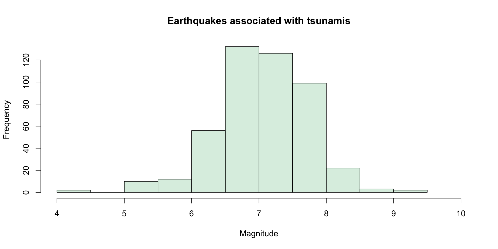
Histograms
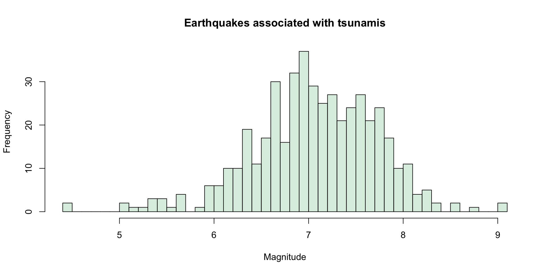
Time plots